Understanding Quality Coefficient and Equivalent Electrical Diagrams

A real coil is never just a coil. A real capacitor is never just a capacitor. Every physical part in an electrical circuit carries hidden resistance, leakage, capacitance, inductance, heat loss, and frequency-dependent behavior.
That is why two ideas matter so much in circuit analysis: quality coefficient, often called the Q factor, and equivalent electrical diagrams. One tells us how “clean” or selective an energy-storing system is. The other gives us a useful model for parts that are more complicated than their symbol suggests.
Together, they help explain why a radio tuner can select one station and reject another, why a filter has a sharp or gentle response, why an inductor heats up, and why a capacitor stops behaving ideally at high frequency.

What the quality coefficient measures
The quality coefficient, usually written as Q, measures how efficiently a circuit or component stores energy compared with how much energy it loses.
A high-Q system stores energy well and loses little energy per cycle. A low-Q system loses energy quickly.
In electrical circuits, Q appears most often in systems that exchange energy between electric and magnetic fields, such as:
LC resonant circuits
RLC filters
Inductors
Capacitors
Crystal resonators
Antennas
Tuned radio circuits
A simple way to describe Q is:
\[
Q = 2\pi \times \frac{\text{energy stored}}{\text{energy lost per cycle}}
\]
This definition applies broadly. It does not depend on one specific circuit shape. It says that Q compares stored energy with wasted energy.
In a resonant circuit, energy moves back and forth. The capacitor stores energy in an electric field. The inductor stores energy in a magnetic field. Resistance turns part of that energy into heat. Q describes how many cycles the energy can “ring” before it fades.
A high-Q circuit rings for a long time. A low-Q circuit dies out quickly.
A mechanical comparison makes Q easier to picture
Imagine a swing.
If the swing has little friction, one push keeps it moving for a long time. That is a high-Q system.
If the swing has strong friction, it stops after only a few passes. That is a low-Q system.
Electrical resonance behaves in a similar way. The inductor and capacitor trade energy, while resistance drains energy from the system.
The greater the losses, the lower the Q.
Q and resonance are closely linked
Resonance occurs when inductive reactance and capacitive reactance balance each other. At that frequency, a circuit can store and exchange energy very effectively.
For an ideal LC circuit, the resonant frequency is:
\[
f_0 = \frac{1}{2\pi\sqrt{LC}}
\]
Where:
\( f_0 \) is resonant frequency in hertz
\( L \) is inductance in henries
\( C \) is capacitance in farads
In the real world, resistance always appears somewhere. It may come from the wire in an inductor, dielectric loss in a capacitor, contact resistance, skin effect, core loss, or connected load. That resistance controls the Q.
For a series RLC circuit, the quality coefficient at resonance is commonly written as:
\[
Q = \frac{\omega_0 L}{R}
\]
or:
\[
Q = \frac{1}{\omega_0 C R}
\]
Where:
\( \omega_0 = 2\pi f_0 \)
\( R \) is the series resistance
\( L \) is inductance
\( C \) is capacitance
These formulas show a direct relationship: higher resistance lowers Q.
For a parallel RLC circuit, the form changes because resistance sits in parallel:
\[
Q = \frac{R}{\omega_0 L}
\]
or:
\[
Q = \omega_0 C R
\]
In this case, a larger parallel resistance means fewer losses, so Q increases.
The exact formula depends on the circuit model. The concept stays the same: Q rises when stored energy dominates loss.

How Q shapes real circuit behavior
Q is not just a theoretical number. It changes what a circuit does.
The most common effects appear in bandwidth, selectivity, damping, voltage magnification, and component heating.
Bandwidth and selectivity
In a resonant circuit, Q relates directly to bandwidth.
\[
Q = \frac{f_0}{BW}
\]
Where:
\( f_0 \) is the center or resonant frequency
\( BW \) is the bandwidth between the half-power points
A high-Q circuit has a narrow bandwidth. It responds strongly near one frequency and weakly away from it.
A low-Q circuit has a wider bandwidth. It responds over a broader range.
This matters in radio receivers. A tuned circuit should accept the desired frequency while rejecting nearby signals. A higher Q gives a sharper selection.
It also matters in filters. A narrow band-pass filter needs a higher Q. A broad tone-control circuit may use a lower Q.
Here is the basic pattern:
Q level | Bandwidth | Response | Common result |
Low Q | Wide | Gentle | Broad filtering, less ringing |
Medium Q | Moderate | Balanced | General tuned circuits |
High Q | Narrow | Sharp | Selective filtering, stronger ringing |
A high Q is not always better. If a signal changes quickly, an overly high-Q circuit may respond too slowly or ring too much. Good design matches Q to the job.
Damping and transient response
Damping describes how quickly oscillations fade.
A low-resistance resonant circuit has low damping and high Q. It keeps oscillating after excitation. This can cause ringing in filters, amplifiers, switching circuits, and transmission lines.
A high-resistance circuit has stronger damping and lower Q. It settles faster but has less selectivity.
This tradeoff appears often:
High Q
Low Q
Narrow response, strong peak, more ringing, lower loss
Broad response, smaller peak, faster settling, higher loss
In digital circuits, ringing can distort edges and cause false switching. In audio circuits, ringing can color the sound. In RF circuits, selective resonance can be useful. The same property can be helpful or harmful depending on context.
Voltage and current magnification
At resonance, energy moves between the inductor and capacitor. In a high-Q series resonant circuit, the voltage across the inductor or capacitor can be much larger than the source voltage.
This surprises many beginners. The source may be only a few volts, yet reactive components can see much higher voltages. That happens because the circuit circulates energy internally.
For this reason, designers check component voltage ratings in resonant circuits. A capacitor in a high-Q tank circuit may face more stress than the supply voltage suggests.
In parallel resonant circuits, circulating currents inside the tank can also be high. The supply sees a high impedance at resonance, but the inductor and capacitor trade significant current.
Losses, heat, and component limits
Q also tells us about component quality.
For an inductor, losses may come from:
Winding resistance
Magnetic core losses
Skin effect at higher frequency
Proximity effect between turns
Radiation or shielding losses
For a capacitor, losses may come from:
Equivalent series resistance
Dielectric absorption
Insulation leakage
Lead inductance
Heating under AC current
Manufacturers often specify Q or dissipation factor for capacitors and inductors. For capacitors, dissipation factor is often the inverse of Q:
\[
DF = \frac{1}{Q}
\]
A low dissipation factor means a high Q. A high dissipation factor means more loss.
This is why part selection matters. A capacitor that works well at low frequency may perform poorly in an RF circuit. An inductor with the right inductance value may still have too much resistance for a high-Q filter.
Why equivalent electrical diagrams are useful
An equivalent electrical diagram represents a real device with ideal circuit elements. It replaces a messy physical object with a model that is easier to analyze.
The word “equivalent” does not mean identical in every possible way. It means equivalent for a chosen purpose, frequency range, signal level, or operating condition.
A real component has many physical effects at once. An equivalent diagram decides which effects matter and shows them with familiar elements such as:
Ideal voltage sources
Ideal current sources
Resistors
Capacitors
Inductors
Dependent sources
Diodes or switches, when needed
The goal is practical analysis. A model should be simple enough to use and accurate enough to trust.
The ideal symbol is only the starting point
Circuit diagrams often begin with ideal symbols.
An ideal resistor has only resistance. An ideal capacitor has only capacitance. An ideal inductor has only inductance.
Real parts do more.
A real resistor has a small inductance because its body and leads form a current path. It may also have small capacitance between its terminals. At low frequency, those effects may not matter. At high frequency, they can change the behavior.
A real capacitor has capacitance, but it also has equivalent series resistance, called ESR, and equivalent series inductance, called ESL. It may also have leakage resistance across the dielectric.
A basic capacitor equivalent diagram may look like this in concept:
```text
ESR ESL C
---/\/\/\/\----LLLLL----||----
|
| leakage path often modeled separately
```
A more complete model may place a large leakage resistance in parallel with the capacitor.
This model explains why capacitors stop looking capacitive at very high frequencies. At some point, the lead and internal inductance dominate. The capacitor can pass through a self-resonant frequency, then begin to behave more like an inductor.
Common equivalent models
Different devices call for different models.
Real item | Simple equivalent diagram | What the model explains |
Battery | Ideal voltage source plus series resistance | Voltage drop under load |
Capacitor | Capacitance plus ESR, ESL, and leakage resistance | Heating, ripple current, high-frequency limits |
Inductor | Inductance plus winding resistance and parasitic capacitance | Q, self-resonance, power loss |
Transformer | Ideal transformer plus winding resistance, leakage inductance, magnetizing inductance, and core loss resistance | Regulation, losses, bandwidth |
Diode | Ideal diode plus voltage drop, series resistance, and junction capacitance | Forward conduction and switching behavior |
Transmission line | Distributed inductance and capacitance with resistance and conductance | Delay, impedance, reflections |
The model grows as the situation demands. A battery powering a small LED may only need an ideal voltage source and one resistor. A battery in a high-current pulse system may need more detail, such as internal resistance, capacitance, and state-of-charge behavior.
Equivalent diagrams depend on frequency
Frequency changes everything.
At DC, a capacitor acts like an open circuit after it charges. An inductor acts like a short circuit after current settles.
At higher frequency, capacitors pass current more easily and inductors oppose changes more strongly. Parasitic effects also become larger.
This means one component can need different equivalent diagrams for different frequency ranges.
For example, a ceramic capacitor used for power-supply bypassing may work well near a digital chip at certain frequencies. At frequencies above its self-resonance, its ESL can reduce its usefulness. Designers often use several capacitors of different values and packages because each one works best over a different range.
This is also why physical layout matters. A perfect schematic on paper can fail in hardware if the traces add unwanted inductance or capacitance.
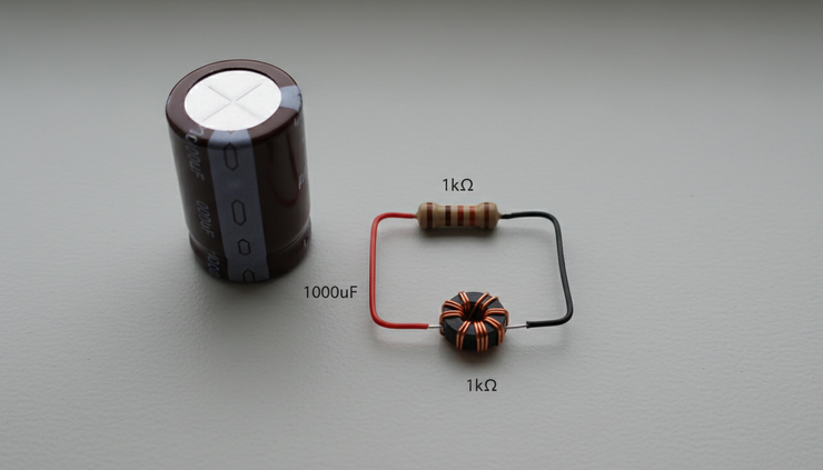
How quality coefficient and equivalent diagrams connect
Q and equivalent diagrams are not separate ideas. Q often comes directly from the equivalent model.
A real inductor, for example, can be modeled as an ideal inductance \(L\) in series with a winding resistance \(R_s\). At a chosen angular frequency \( \omega \), its quality coefficient is:
\[
Q = \frac{\omega L}{R_s}
\]
This equation uses the equivalent diagram. Without the resistance in the model, the inductor would be ideal and its Q would be infinite. That cannot describe a real part.
The same idea applies to a capacitor. A capacitor with equivalent series resistance has:
\[
Q = \frac{1}{\omega C R_s}
\]
Again, the Q depends on the loss element in the equivalent model.
Example using a real inductor model
Suppose an inductor has:
Inductance of \(10 \mu H\)
Series resistance of \(0.5 \Omega\)
Operating frequency of \(1 MHz\)
The angular frequency is:
\[
\omega = 2\pi f = 2\pi \times 1,000,000
\]
The Q is:
\[
Q = \frac{\omega L}{R_s}
\]
\[
Q = \frac{2\pi \times 1,000,000 \times 10 \times 10^{-6}}{0.5}
\]
\[
Q \approx 126
\]
That is a fairly high Q for many practical uses. It means the inductor stores much more energy than it loses per cycle at that frequency.
If the resistance were \(2 \Omega\), the Q would drop to about 31. The inductance did not change. The loss did.
This simple example shows why equivalent diagrams matter. The ideal inductor symbol hides the resistance. The equivalent model reveals it. Q measures the result.
Example using a capacitor model
Suppose a capacitor has:
Capacitance of \(100 nF\)
ESR of \(0.1 \Omega\)
Operating frequency of \(100 kHz\)
The Q is:
\[
Q = \frac{1}{\omega C R_s}
\]
\[
Q = \frac{1}{2\pi \times 100,000 \times 100 \times 10^{-9} \times 0.1}
\]
\[
Q \approx 159
\]
At that frequency, this model suggests low loss. At a much higher frequency, ESL may become important, and the simple ESR-plus-C model may no longer be enough.
That is a key point: a Q value is meaningful only with its frequency and model context.
Why the same part can have different Q values
A component does not always have one fixed Q. Q can change with frequency, temperature, signal level, and construction.
An inductor may lose more energy at high frequency because of skin effect and core loss. A capacitor’s ESR may vary with frequency and temperature. A ferrite-core part may have different losses depending on flux level.
For this reason, datasheets may give Q at a specific test frequency. If the circuit operates far from that test condition, the listed Q may not predict performance well.
Equivalent electrical diagrams help by making those conditions visible. A simple model may use a constant resistance. A better model may use frequency-dependent resistance, parasitic capacitance, or a core-loss branch.
The right model depends on the question being asked.
How to read and build equivalent electrical diagrams
Building an equivalent diagram starts with a practical question.
Do you need to know DC voltage drop? High-frequency noise? Power loss? Resonance? Switching speed? Thermal stress?
The answer decides which effects belong in the model.
Start with the dominant ideal behavior
Begin with the main function of the part.
A resistor starts as resistance.
A capacitor starts as capacitance.
An inductor starts as inductance.
A battery starts as a voltage source.
A transformer starts as magnetic coupling.
This ideal model gives the first approximation.
For many low-speed circuits, it may be enough. A pull-up resistor in a simple digital input usually does not need a detailed parasitic model. A timing capacitor in a low-frequency circuit may only need capacitance and leakage.
Good modeling does not mean adding every possible effect. It means adding the effects that change the answer.
Add loss elements
Next, add the losses.
Loss often appears as resistance, but placement matters.
Series resistance represents losses in the current path. This model works well for wire resistance, ESR, and winding resistance.
Parallel resistance represents leakage or shunt loss. This model works well for insulation leakage, dielectric loss in some cases, or core loss branches in transformer models.
For a capacitor, leakage resistance usually appears in parallel with the capacitance. ESR appears in series.
For an inductor, winding resistance often appears in series. Core loss may appear as a parallel resistance in some AC models.
These choices are not arbitrary. They reflect the physical path where energy is lost.
Add parasitic storage elements
After losses, add unwanted capacitance or inductance.
A long wire has inductance. Two nearby conductors have capacitance. A resistor has lead inductance. An inductor has turn-to-turn capacitance. A capacitor has lead inductance.
At low frequency, these effects may be tiny. At high frequency, they can dominate.
This is why RF circuits often look strange to people used to DC circuits. Wires are no longer just connections. They become circuit elements.
A short trace can add enough inductance to reduce bypass capacitor performance. A nearby ground plane can add capacitance. A connector can introduce reflections. An equivalent diagram gives those effects a place in the analysis.
Check the model against the operating range
Every model has limits.
A model that works at 1 kHz may fail at 100 MHz. A model that works for small signals may fail when the core saturates or the diode switches hard. A model that works at room temperature may shift when the part heats.
A useful equivalent diagram should state, at least mentally:
The frequency range
The signal size
The temperature range
The operating mode
The accuracy needed
If those conditions change, the model may need to change.
Use measurement when possible
Measurements can confirm or adjust a model.
Common tools include:
Digital multimeter for DC resistance and voltage
LCR meter for inductance, capacitance, resistance, Q, and dissipation factor
Oscilloscope for ringing, damping, and transient response
Signal generator for frequency response
Network analyzer for impedance and scattering parameters at higher frequencies
A measured resonance peak can reveal Q. A decaying waveform can show damping. An impedance plot can show self-resonance.
The best circuit understanding often comes from moving between three views:
The physical part
The equivalent diagram
The measured behavior
When all three agree closely enough, the model is doing its job.

Common mistakes when using Q and equivalent diagrams
The ideas are simple, but mistakes happen often.
Treating ideal symbols as real parts
The ideal schematic is not the full truth. It is a starting point.
A power supply bypass capacitor with long leads may not suppress fast noise well. An inductor with high winding resistance may fail in a selective filter. A transformer model without leakage inductance may miss voltage spikes.
When a circuit behaves strangely, the missing parasitic element is often the clue.
Ignoring the frequency attached to Q
A Q rating without frequency has limited value.
An inductor might have a high Q at one frequency and a lower Q at another. A capacitor might work well below self-resonance and poorly above it.
Always ask: measured or calculated at what frequency?
Using a model outside its range
Equivalent diagrams are tools, not permanent identities.
A battery modeled as an ideal source plus series resistance may work for simple load calculations. It may not describe fast pulses, aging, temperature effects, or electrochemical recovery.
A diode model with a fixed voltage drop may work for rough DC estimates. It may not predict switching loss or high-speed behavior.
Use the simplest model that answers the question, but no simpler.
Assuming higher Q is always better
High-Q circuits are selective and efficient, but they can ring. They may create high internal voltages or currents. They can be sensitive to component tolerance and temperature drift.
Low-Q circuits waste more energy, but they settle faster and behave more broadly.
The best Q is the one that fits the circuit’s purpose.
A practical way to put the concepts together
When analyzing a real circuit, use this short process:
Identify the energy storage elements.
Look for inductors, capacitors, transmission lines, crystals, transformers, and parasitic fields.
Identify the loss paths.
Find winding resistance, ESR, leakage, load resistance, core loss, radiation, and switching loss.
Draw the simplest equivalent diagram that includes those effects.
Calculate or estimate Q at the operating frequency.
Compare the predicted behavior with the real circuit.
Look for bandwidth, ringing, heating, resonance, and voltage stress.
Refine the model only if the first version does not explain what you see.
This process keeps analysis grounded. It avoids both extremes: pretending parts are ideal, or building a model so complex that it becomes unusable.
Quality coefficient gives a number to energy loss. Equivalent electrical diagrams show where that loss comes from. Once those two ideas connect, circuits become easier to predict, troubleshoot, and design.
The symbol on a schematic may look simple, but the real part always has a story. Q helps measure that story. The equivalent diagram helps tell it.


Comments